
HAMUX
A New Class of Deep Learning Library Built around ENERGY
Part proof-of-concept, part functional prototype, HAMUX is designed to bridge modern AI architectures and Hopfield Networks.
HAMUX: A Hierarchical Associative Memory User eXperience.
🚧 HAMUX is in rapid development. Remember to specify the version when building off of HAMUX.
A Universal Abstraction for Hopfield Networks
HAMUX fully captures the the energy fundamentals of Hopfield Networks and enables anyone to:
🧠 Build DEEP Hopfield nets
🧱 With modular ENERGY components
🏆 That resemble modern DL operations
Every architecture built using HAMUX is a dynamical system guaranteed to have a tractable energy function that converges to a fixed point. Our deep Hierarchical Associative Memories (HAMs) have several additional advantages over traditional Hopfield Networks (HNs):
| Hopfield Networks (HNs) | Hierarchical Associative Memories (HAMs) |
|---|---|
| HNs are only two layers systems | HAMs connect any number of layers |
| HNs model only simple relationships between layers | HAMs model any complex but differentiable operation (e.g., convolutions, pooling, attention, \(\ldots\)) |
| HNs use only pairwise synapses | HAMs use many-body synapses (which we denote HyperSynapses) |
How does HAMUX work?
HAMUX is a hypergraph of 🌀neurons connected via 🤝hypersynapses, an abstraction sufficiently general to model the complexity of connections used in modern AI architectures.
We conflate the terms hypersynapse and synapse regularly. We explicitly say "pairwise synapse" when referring to the classical understanding of synapses.
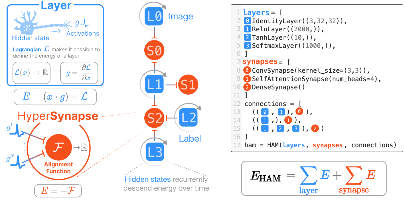
HAMUX defines two fundamental building blocks of energy: the 🌀neuron layer and the 🤝hypersynapse (an abstraction of a pairwise synapse to include many-body interactions) connected via a hypergraph. It is a fully dynamical system, where the “hidden state” \(x_i^l\) of each layer \(l\) (blue squares in the figure below) is an independent variable that evolves over time. The update rule of each layer is entirely local; only signals from a layer’s connected synapses (red circles in the figure below) can tell the hidden state how to change. This is shown in the following equation:
\[\tau \frac{d x_{i}^{l}}{dt} = -\frac{\partial E}{\partial g_i^l}\]
where \(g_i^l\) are the activations (i.e., non-linearities) on each neuron layer, described in the section on Neuron Layers. Concretely, we implement the above differential equation as the following discretized equation (where the bold \({\mathbf x}_l\) is the collection of all elements in layer \(l\)’s state):
\[ \mathbf{x}_l^{(t+1)} = \mathbf{x}_l^{(t)} - \frac{dt}{\tau} \nabla_{\mathbf{g}_l}E(t)\]
HAMUX handles all the complexity of scaling this fundamental update equation to many layers and hyper synapses. In addition, it provides a framework to:
- Implement your favorite Deep Learning operations as a HyperSynapse
- Port over your favorite activation functions as Lagrangians
- Connect your layers and hypersynapses into a HAM (using a hypergraph as the data structure)
- Inject your data into the associative memory
- Automatically calculate and descend the energy given the hidden states at any point in time
Use these features to train any hierarchical associative memory on your own data! All of this made possible by JAX.
The examples/ subdirectory contains a (growing) list of examples on how to apply HAMUX on real data.
🌀Neuron Layers
Neuron layers are the recurrent unit of a HAM; that is, 🌀neurons keep a state that changes over time according to the dynamics of the system. These states always change to minimize the global energy function of the system.
For those of us familiar with traditional Deep Learning architectures, we are familiar with nonlinear activation functions like the ReLU and SoftMax. A neuron layer in HAMUX is exactly that: a nonlinear activation function defined on some neuron. However, we need to express the activation function as a convex Lagrangian function \(\mathcal{L}\) that is the integral of the desired non-linearity such that the derivative of the Lagrangian function \(\nabla \mathcal{L}\) is our desired non-linearity. E.g., consider the ReLU:
\[ \begin{align*} \mathcal{L}(x) &:= \frac{1}{2} (\max(x, 0))^2\\ \nabla \mathcal{L} &= \max(x, 0) = \mathrm{relu}(x)\\ \end{align*} \]
We need to define our activation layer in terms of the Lagrangian of the ReLU instead of the ReLU itself. Extending this constraint to other nonlinearities makes it possible to define the scalar energy for any neuron in a HAM. It turns out that many activation functions used in today’s Deep Learning landscape are expressible as a Lagrangian. HAMUX is “batteries-included” for many common activation functions including relus, softmaxes, sigmoids, LayerNorms, etc. See our documentation on Lagrangians for examples on how to implement efficient activation functions from Lagrangians in JAX. We show how to turn Lagrangians into usable energy building blocks in our documentation on neuron layers.
🤝HyperSynapses
A 🤝hypersynapse ONLY sees activations of connected 🌀neuron layers. Its one job: report HIGH ⚡️energy if the connected activations are dissimilar and LOW ⚡️energy when they are aligned. Hypersynapses can resemble convolutions, dense multiplications, even attention… Take a look at our documentation on (hyper)synapses.
🚨 Point of confusion: modern AI frameworks have
ConvLayers and NormalizationLayers. In HAMUX, these would be more appropriately called ConvSynapses and NormalizationLagrangians.
Install
From pip:
pip install hamuxIf you are using accelerators beyond the CPU you will need to additionally install the corresponding jax and jaxlib versions following their documentation. E.g.,
pip install --upgrade "jax[cuda]" -f https://storage.googleapis.com/jax-releases/jax_cuda_releases.htmlFrom source:
After cloning:
cd hamux
conda env create -f environment.yml
conda activate hamux
pip install --upgrade "jax[cuda]" -f https://storage.googleapis.com/jax-releases/jax_cuda_releases.html # If using GPU accelerator
pip install -e .
pip install -r requirements-dev.txt  # To run the examples
How to Use
import hamux as hmx
import jax.numpy as jnp
import jax
import jax.tree_util as jtu
We can build a simple 4 layer HAM architecture using the following code
layers = [
    hmx.TanhLayer((32,32,3)), # e.g., CIFAR Images
    hmx.SigmoidLayer((11,11,1000)), # CIFAR patches
    hmx.SoftmaxLayer((10,)), # CIFAR Labels
    hmx.SoftmaxLayer((1000,)), # Hidden Memory Layer
]

synapses = [
    hmx.ConvSynapse((3,3), strides=3),
    hmx.DenseSynapse(),
    hmx.DenseSynapse(),
]

connections = [
    ([0,1], 0),
    ([1,3], 1),
    ([2,3], 2),
]

rng = jax.random.PRNGKey(0)
param_key, state_key, rng = jax.random.split(rng, 3)
states, ham = hmx.HAM(layers, synapses, connections).init_states_and_params(param_key, state_key=state_key);
Notice that we did not specify any output channel shapes in the synapses. The desired output shape is computed from the layers connected to each synapse during hmx.HAM.init_states_and_params.
We have two fundamental objects: states and ham. The ham object contains the connectivity structure of the HAM (e.g., layer+hypersynapse+hypergraph information) alongside the parameters of the network. The states object is a list of length nlayers where each item is a tensor representing the neuron states of the corresponding layer.
assert len(states) == ham.n_layers
assert all([state.shape == layer.shape for state, layer in zip(states, ham.layers)])
We make it easy to run the dynamics of any HAM. Every forward function is defined external to the memory and can be modified to extract different memories from different layers, as desired. The general steps for any forward function are:
- Initialize the dynamic states
- Inject an initial state into the system
- Run dynamics, calculating energy gradient at every point in time.
- Return the layer state/activation of interest
def fwd(model, x, depth=15, dt=0.1):
    """Assuming a trained HAM, run association with the HAM on batched inputs `x`"""
    # 1. Initialize model states at t=0. Account for batch size
    xs = model.init_states(x.shape[0])

    # Inject initial state
    xs[0] = x

    energies = []
    for i in range(depth):
        energies.append(model.venergy(xs)) # If desired, observe the energy
        dEdg = model.vdEdg(xs)  # Calculate the gradients
        xs = jtu.tree_map(lambda x, stepsize, grad: x - stepsize * grad, xs, model.alphas(dt), dEdg)


    # Return probabilities of our label layer
    probs = model.layers[-2].activation(xs[-2])
return jnp.stack(energies), probsbatch_size=3
x = jax.random.normal(jax.random.PRNGKey(2), (batch_size, 32,32,3))
energies, probs = fwd(ham, x, depth=20, dt=0.3)
print(probs.shape) # batchsize, nclasses
assert jnp.allclose(probs.sum(-1), 1)(3, 10)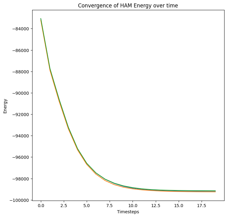
More examples coming soon!
The Energy Function vs the Loss Function
We use JAX’s autograd to descend the energy function of our system AND the loss function of our task. The derivative of the energy is always taken wrt to our states; the derivative of the loss function is always taken wrt our parameters. During training, we change our parameters to optimize the Loss Function. During inference, we assume that parameters are constant.
Autograd for Descending Energy
Every HAM defines the energy function for our system, which is everything we need to compute memories of the system. Naively, we can calculate \(\nabla_x E\): the derivative of the energy function wrt the states of each layer:
stepsize = 0.01
fscore_naive = jax.grad(ham.energy)
next_states = jax.tree_util.tree_map(lambda state, score: state - stepsize, states, fscore_naive(states))
But it turns out we improve the efficiency of our network if we instead take \(\nabla_g E\): the derivative of the energy wrt the activations instead of the states. They have the same local minima, even though the trajectory to get there is different. Some nice terms cancel, and we get:
\[\nabla_g E_\text{HAM} = x + \nabla_g E_\text{synapse}\]
stepsize = 0.01
def fscore_smart(xs):
    gs = ham.activations(xs)
    return jax.tree_util.tree_map(lambda x, nabla_g_Esyn: x + nabla_g_Esyn, xs, jax.grad(ham.synapse_energy)(gs))

next_states = jax.tree_util.tree_map(lambda state, score: state - stepsize, states, fscore_smart(states))
Credits
Read our extended abstract on OpenReview: HAMUX: A Universal Abstraction for Hierarchical Hopfield Networks
Work is a collaboration between the MIT-IBM Watson AI Lab and the PoloClub @ GA Tech. - Ben Hoover (IBM & GATech) - Polo Chau (GATech) - Hendrik Strobelt (IBM) - Dmitry Krotov (IBM)